Kalman filters
- Introduction
- Filtering, smoothing, prediction
- Why filter?
- Covariance
- a priori, a posteriori
- Properties - predominant
- Simulation
- References
Introduction
The Kalman filter is essentially a set of mathematical equations that implement a predictor-corrector type estimator that is optimal in the sense that it minimizes the estimated error covariance
Filtering, smoothing, prediction
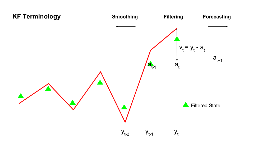
- Filtering is an estimation problem where all the observations upto time N are used to get a best estimate at time N itself (k = N)
- Smoothing is given a set of observations from 1 to N, estimate a state at the time in past
- Prediction is an estimation problem where all the observations upto time N are used to get a best estimate at time (N+1)
Mathematically, \(F_N =z_i \mid 1 \leqslant i \leqslant N\) where k < N (smoothing), k = N (filtering) and k > N (prediction)
Why "filter"?
You might be wondering, why the word “filter” used?
The process of finding the “best estimate” from noisy data amounts to “filtering out” the noise. However, kalman filter also doesn’t just clean up the data measurements, but also projects these measurements onto the state estimate.
Covariance
Covariance: In probability, covariance is the measure of the joint probability for two random variables. It describes how the two variables change together. \(cov(X, Y) = E[(X - E[X]) . (Y - E[Y])]\). The sign of the covariance can be interpreted as whether the two variables increase together (positive) or decrease together (negative). The magnitude of the covariance is not easily interpreted. A covariance value of zero indicates that both variables are completely independent.
Covariance matrix: A matrix where diagonal elements are the variances, off-diagonal encode correlations. It is symmetric (since cov(x,y) = cov(y,x))
a priori, a posteriori
\(\hat{x_k^\prime}\) is a priori state estimate at step k given knowledge of the process prior to step k, and \(\hat{x_k}\) is a posteriori state estimate at step k given measurement \(z_k\). a priori and a posteriori estimate errors are defined as \(e_k^\prime = x_k - \hat{x_k}^\prime\) and \(e_k = x_k - \hat{x_k}\). The a prior estimate error covariance is \(P_k^\prime = E[e_k^\prime e_k^{\prime T}]\) and the a posteriori estimate error covariance is \(P_k = E[e_k e_k^{T}]\).
Properties
- Kalman filters bear the following properties:
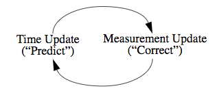
- They belong to a class of problems called predictor-corrector algorithms, where they proceed in two steps:
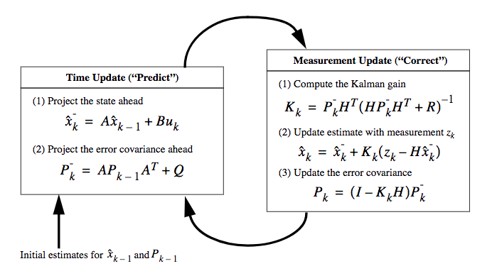
- Time update step: They are responsible for projecting forward (in time) the current state and error covariance estimates to obtain the a priori estimates for the next time step.
- Measurement update step: They are responsible for the feedback—i.e. for incorporating a new measurement into the a priori estimate to obtain an improved a posteriori estimate
- They belong to the class of linear methods, since the underlying filtering model is linear and the distributions are assumed Gaussian
- They are optimal estimators, since they infer parameters of interest from indirect, inaccurate and uncertain observations.
- They are recursive and requires only the last “best guess”, rather than the entire history, of a system’s state to calculate a new state.
- They address the general problem of trying to estimate the state of a discrete-time controlled process that is governed by a linear stocastic difference equation. If the process to be estimated or the measurement relationship to the process non-linear, use extended kalman filter
- They are similar to Hidden Markov Model (HMMs) except, the state space of latent variables (hidden variable) is continuos and all latent and observed variables have gaussian distributions.
- They produce an estimate of the state of the system as an average of the system’s predicted state (\(\hat{x_k}^\prime\)) and of the new measurement (\(z_k\)) using a weighted average (also called kalman gain, \(K_k\)). The result of the weighted average is a new state estimate that lies between the predicted and measured state, and has a better estimated uncertainty than either alone. This process is repeated at every time step, with the new estimate and its covariance informing the prediction used in the following iteration.
- The relative certainty of the measurements (\(z_k\)) and current state estimate (\(\hat{x_k}^\prime\)) is an important consideration, and it is common to discuss the response of the filter in terms of the kalman filter’s gain. The kalman gain is the relative weight given to the measurements and current state estimate, and can be tuned to achieve particular performance. With a high gain, the filter places more weight on the most recent measurements, and thus follows them more responsively. With a low gain, the filter follows the model predictions more closely. At the extremes, a high gain close to 1 will result in a more jumpy estimated trajectory, while low gain close to 0 will smooth out noise but decrease the responsiveness.
- Looking at kalman gain equation, i.e it is evident that, as the measurement error covariance R approaches zero, the gain K weights the residual more heavily. On the other hand, as the a priori estimate error covariance \({P^\prime}_k\) approaches zero, the gain \(K\) weights the residual less heavily. Another way of thinking about the weighting by \(K\) is that as the measurement error covariance \(R\) approaches zero, the actual measurement \(z_k\) is “trusted” more and more, while the predicted measurement \(H\hat{x_k}^\prime\) is trusted less and less. On the other hand,as the a priori estimate error covariance \({P^\prime}_k\) approaches zero the actual measurement \(z_k\) is trusted less and less, while the predicted measurement \(H\hat{x_k}^\prime\) is trusted more and more.
- The innovation/residual is the difference between the observed value of a variable at time t (\(z_k\)) and the optimal forecast of that value based on information available prior to time t (\(H\hat{x_k}^\prime\)). A residual of zero means that the two are in complete agreement.
- They belong to a class of problems called predictor-corrector algorithms, where they proceed in two steps:
- After each time and measurement update pair, the process is repeated with the previous a posteriori estimates used to project or predict the new a priori estimates. This recursive nature is one of the very appealing features of the Kalman filter—it makes practical implementations much more feasible than (for example) an implementation of a Wiener filter (Brown and Hwang 1996) which is designed to operate on all of the data directly for each estimate.
Simulation
To begin with the simulation, i.e  at t=0, “seed” our filter with the guess that the constant is 0. In other words, before starting we let \(xhat_{k-1} = 0\). Similarly, we need to choose an initial value for \(P_{k-1}\), call it \(P_0\). If we were absolutely certain that our initial state estimate \(\hat{x}_0 = 0\) was correct, we would let \(P_0 = 0\). However given the uncertainty in our initial estimate \(\hat{x}_0 = 0\) , choosing \(P_0 = 0\) would cause the filter to initially and always believe \(\hat{x}_0 = 0\). As it turns out, the alternative choice is not critical. We could choose almost any \(P_0 \neq 0\) and the filter would eventually converge. We’ll start our filter with \(P_0 = 1\)
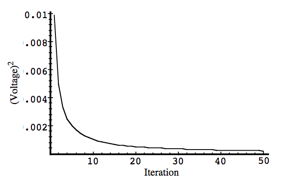
We will carry out 3 simulations, with \(R = 0.01, R = 1, R = 0.00001\)
Simulation 1
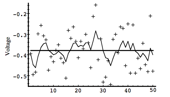
In the first simulation we fixed the measurement variance at \(R = (0.1)^2 = 0.01\). Because this is the “true” measurement error variance, we would expect the “best” performance in terms of balancing responsiveness and estimate variance. It will balance itself out in the second and third simulation (takes time for stabilization).
Simulation 2
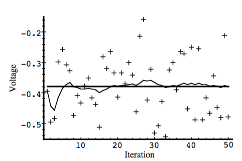
If the measurement covariance(R) is high, (R = 1) it was “slower” to respond to the measurements (similar to learning rate), resulting in reduced estimate variance (smooth curve)
Simulation 3
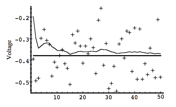
In the below figure, the filter was told the measurement variance is (R = 0.00001), it was very “quick” to believe the noisy measurements
